Alexander Neiman, Lutz Schimansky-Geier
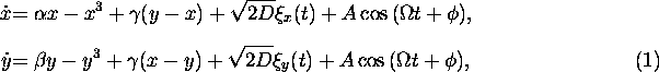
We consider the collective response on a periodical force of two coupled bistable oscillators driven by independent noise sources. We have found that there exist an optimal value of coupling strength at which the signal-to-noise ratio of the collective response takes its maximal value. The connection of this effect with the phenomenon of stochastic synchronization is established.
Recently the phenomenon of stochastic resonance (SR) [1] became an attractor of extensive investigations in the field of nonlinear stochastic systems. There are a lot of theoretical work, numerical and analog simulations [2]. The SR has been observed in laser [3], in paramagnetic systems [4], during ion transport through channels of cell membranes [5]. Of high interest are investigations concerned with this phenomenon in biological systems in view of sensory neuron activity and neuron networks [6]. For these investigations studies of coupled oscillators are of high relevance.
In recent papers [7]-[8] the SR in globally coupled bistable oscillators were studied. Using a mean field approach [7] and eliminating adiabatically the bath variables [8] an increase of the signal-to-noise ratio (SNR) was found.
For a better understanding of coupled bistable systems we consider in the present paper only two systems, bistable and coupled but with different Kramers-escape times [9]. Recently we have shown that in such systems synchronization-like phenomena (which was called stochastic synchronization) can be observed [10].
We consider two mutually coupled bistable overdamped oscillators which are forced by statistically independent noises and one periodical signal. The system under consideration is governed by the following stochastic differential equations
where ![]() and
and ![]() are the parameters which determine the Kramers
rates in the subsystems;
are the parameters which determine the Kramers
rates in the subsystems; ![]() is the strength of coupling and
D is the intensity of the zero-mean white Gaussian noises
is the strength of coupling and
D is the intensity of the zero-mean white Gaussian noises ![]() and
and ![]() ,
and
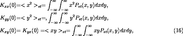
,
and ![]() is the random initial phase of the signal.
is the random initial phase of the signal.
In this physical situation we have to deal with three characteristic
time scales: the period of the external force ![]() and two
different Kramers times of the subsystems,
and two
different Kramers times of the subsystems, ![]() and
and ![]() . The interplay
between them by changing the strength of coupling
. The interplay
between them by changing the strength of coupling ![]() will be the
main interest of our study. We can expect
at least two different mechanisms of growth of coherence which influence
on the stochastic resonance.
First, we observe coherent behavior of the subsystems at the driving
frequency
will be the
main interest of our study. We can expect
at least two different mechanisms of growth of coherence which influence
on the stochastic resonance.
First, we observe coherent behavior of the subsystems at the driving
frequency ![]() only. Lateron we will show the increase of coherence due to
coupling at
only. Lateron we will show the increase of coherence due to
coupling at ![]() .
The second mechanism occurs due to the coupling of the
bistable systems.
This case without periodical forcing, A=0, was considered in [10].
It was shown that by increasing the coupling strength
x(t) and y(t) become coherent, i.e. the coherence function
.
The second mechanism occurs due to the coupling of the
bistable systems.
This case without periodical forcing, A=0, was considered in [10].
It was shown that by increasing the coupling strength
x(t) and y(t) become coherent, i.e. the coherence function ![]()
approaches values near one ( ![]() ) for a wide region
of frequencies. In (2)
) for a wide region
of frequencies. In (2) ![]() is the cross spectrum of the processes x(t),
y(t) and
is the cross spectrum of the processes x(t),
y(t) and ![]() ,
, ![]() are the power spectra of
x(t), y(t), respectively.
Thus, contrary to the first mechanism the second one takes place
for a wide region of frequencies.
The transition to coherent behavior is accompanied by a change of the
modality of the two-dimensional stationary probability density p(x,y). Before this
transition the probability density has four maxima which correspond to
four wells of the appropriate potential. After the transition p(x,y)
possesses two maxima. That circumstance leads to the synchronization of the
processes in the subsystems via locking of their Kramers frequencies
(see Fig.3 and Fig.5 in [10]).
are the power spectra of
x(t), y(t), respectively.
Thus, contrary to the first mechanism the second one takes place
for a wide region of frequencies.
The transition to coherent behavior is accompanied by a change of the
modality of the two-dimensional stationary probability density p(x,y). Before this
transition the probability density has four maxima which correspond to
four wells of the appropriate potential. After the transition p(x,y)
possesses two maxima. That circumstance leads to the synchronization of the
processes in the subsystems via locking of their Kramers frequencies
(see Fig.3 and Fig.5 in [10]).
We interest in the collective behaviour of the system. It can be described by introducing the new variable
The power spectrum of the collective output u(t) reads
Here ![]() is the real part of the cross spectrum
and appears from the correlations between x(t) and y(t). It will be
remarkabely depend on the degree of coherence.
is the real part of the cross spectrum
and appears from the correlations between x(t) and y(t). It will be
remarkabely depend on the degree of coherence.
As in any study of stochastic resonance the quantity of interest is the signal-to-noise ratio (SNR) of the collective variable u(t). Let us consider first the special case of monostable coupled systems. The aim to consider monostable systems is to investigate the coherence phenomena of the first type, i.e. at the driving frequency only. We will apply the linear response theory [11], [12], [13].
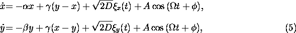
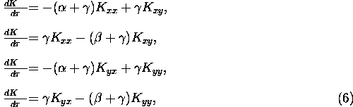
For this purpose it will be sufficient to study coupled sytems with parabolic potential. The dynamics then obeys the system of linear stochastic differential equation
where ![]() and
and ![]() should be positive values.
Obviously, in such systems stochastic resonance will not be observed
(Stochastic
resonance can be observed in underdamped monostable
oscillator [14])
but the SNR at the driving frequency will be of interest. For the correlaton
functions we got the following equations
should be positive values.
Obviously, in such systems stochastic resonance will not be observed
(Stochastic
resonance can be observed in underdamped monostable
oscillator [14])
but the SNR at the driving frequency will be of interest. For the correlaton
functions we got the following equations
which must be solved with initial conditions
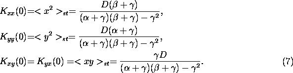
For the correlation function of the collective variable we finally obtain
![]()
where
For the susceptibility [11] of the collective variable u(t) we derive the exact expression
The SNR is connected with the susceptibility ![]() and with the
power spectrum of the unperturbed system
and with the
power spectrum of the unperturbed system ![]() , i.e. in the
absence of periodical excitation. It is defined by the expression
, i.e. in the
absence of periodical excitation. It is defined by the expression
In our particular case for the collective variable u(t) we find
In the Fig.1 the dependence of the SNR of the collective variable
vs the coupling strength ![]() is shown.
The monotonic increase of the SNR reflects the growth
of the coherence by increasing the coupling. We point out that the remaining part
of the spectrum, the noisy contribution, is more or less unaffected by changing
the coupling strength.
is shown.
The monotonic increase of the SNR reflects the growth
of the coherence by increasing the coupling. We point out that the remaining part
of the spectrum, the noisy contribution, is more or less unaffected by changing
the coupling strength.
Now let us consider bistable systems. We start with the limits
![]() ,
, ![]() and
and ![]() .
.
The case ![]() .
The response function of the collective variable in this case
is just the sum of the response functions of the subsystems.
Taking into account, for simplicity, the hoppings between the wells [13] only
we found the susceptibility
.
The response function of the collective variable in this case
is just the sum of the response functions of the subsystems.
Taking into account, for simplicity, the hoppings between the wells [13] only
we found the susceptibility ![]() in the same shape (9) as in the previous case but with another
coefficients.
Now
in the same shape (9) as in the previous case but with another
coefficients.
Now ![]() and
and ![]() are the second order cumulants of the
unperturbed bistable subsystems and
are the second order cumulants of the
unperturbed bistable subsystems and
![]() ,
,
![]() are
the corresponding eigenvalues of the hopping dynamics in the subsystems.
Then for the SNR of the collective variable we obtain again the expression (11)
and for the SNRs of x(t) and y(t):
are
the corresponding eigenvalues of the hopping dynamics in the subsystems.
Then for the SNR of the collective variable we obtain again the expression (11)
and for the SNRs of x(t) and y(t):
In Fig.2 we show the SNRs vs noise intensity of both subsystems separately
(symbols ![]() and
and ![]() ) and of the collective output (symbol
) and of the collective output (symbol ![]() ).
It is seen that
).
It is seen that ![]() takes its maxima approximately at the same
noise intensities as
the SNRs for y(t) and x(t). The region at which the SNR is
maximal becomes wider.
takes its maxima approximately at the same
noise intensities as
the SNRs for y(t) and x(t). The region at which the SNR is
maximal becomes wider.
The case ![]() .
In this case we derive a stochastic differential
equation for the collective variable. It reads
.
In this case we derive a stochastic differential
equation for the collective variable. It reads
and ![]() . Again from the linear response approach
we find the SNR of the collective variable
. Again from the linear response approach
we find the SNR of the collective variable
where ![]() ,
and
,
and ![]() .
The dependence
.
The dependence ![]() is shown in Fig.2 (symbol
is shown in Fig.2 (symbol ![]() ).
We find the usual SNR vs noise intensity. In comparison to the previous case the
maximal SNR is below of the value of the decoupled case. It is important
to point out that the stochastic resonance takes place at the noise intensities
which correspond to the region of the stochastic resonance of the slower dynamics
x(t). That is in agreement with the results of [10] where it was shown
that the strongly coupled bistable systems approaches time scales
of the slower dynamics.
).
We find the usual SNR vs noise intensity. In comparison to the previous case the
maximal SNR is below of the value of the decoupled case. It is important
to point out that the stochastic resonance takes place at the noise intensities
which correspond to the region of the stochastic resonance of the slower dynamics
x(t). That is in agreement with the results of [10] where it was shown
that the strongly coupled bistable systems approaches time scales
of the slower dynamics.
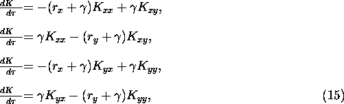
Weak coupling case ![]() . In this case for two-state
dynamics we can write for the correlation functions the following equations
. In this case for two-state
dynamics we can write for the correlation functions the following equations
which must be solved with initial conditions
where ![]() is the stationary probability density of the processes
x(t), y(t) in the absence of periodical excitation [10].
The correlations function of the collective variable follows again (8) with
is the stationary probability density of the processes
x(t), y(t) in the absence of periodical excitation [10].
The correlations function of the collective variable follows again (8) with
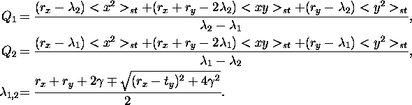
The susceptibility and the signal-to-noise ratio follow (9) and (10) respectively with specified coefficients given above. Calculations in accordance with these expressions showed qualitatively the same behavior as in the case of linear coupled systems: the signal-to-noise ratio grow with increase of the coupling strength (cf. Fig.1).
Thus, we have shown that in the case of strong coupling the signal-to-noise ratio less than in the decoupled case. At the same time for the case of weak coupling we observe an increase of SNR with increase of the coupling strength. Therefore, we can expect exsistence of an optimal value of the coupling strength at which the SNR takes its maximal value.
Let us consider now the case of intermediate values of the coupling strength.
In this case we use numerical simulations to
calculate the SNR.
In Fig.3 we present the SNRs
vs the noise intensity of the subsystems for increasing values of the coupling strength.
It is seen that ![]() reflects the stochastic synchronization of the
processes in the subsystems. In the decoupling case
reflects the stochastic synchronization of the
processes in the subsystems. In the decoupling case ![]() take their maxima
at the noise intensities which correspond to the Kramers rates of the subsystems (Fig.3,a).
With the increase of the coupling strength the Kramers rates in the subsystems tend to
coincide (see Fig.5 in [10]). This reflects in the behaviour of the
take their maxima
at the noise intensities which correspond to the Kramers rates of the subsystems (Fig.3,a).
With the increase of the coupling strength the Kramers rates in the subsystems tend to
coincide (see Fig.5 in [10]). This reflects in the behaviour of the
![]() (Fig.3,b,c). Eventually, the SNRs in both subsystems take their maxima
approximately at the same noise intensity (Fig.3,d).
(Fig.3,b,c). Eventually, the SNRs in both subsystems take their maxima
approximately at the same noise intensity (Fig.3,d).
The behaviour of the collective response is shown in Fig.4.
We plot the dependence of maximal value of the SNR ![]() vs the coupling strength
vs the coupling strength ![]() .
It is important to note that this dependence possesses a maximum. Therefore, there exists
an optimal value of the coupling strength. Otherwise as in the monostable coupled systems
the SNR beyond this value decreases with the increase of the coupling strength.
.
It is important to note that this dependence possesses a maximum. Therefore, there exists
an optimal value of the coupling strength. Otherwise as in the monostable coupled systems
the SNR beyond this value decreases with the increase of the coupling strength.
Let us give now a qualitative explanation of that phenomenon.
As we already mentioned, the power spectrum of the collective variable (4)
contains also the term ![]() .
It is responsible for the coherence between the processes x(t) and y(t) in the subsystems.
The SNR is the relation
of the signal part to the noise part of the spectrum. In both parts we will
find contributions arising from the growth of coherence.
.
It is responsible for the coherence between the processes x(t) and y(t) in the subsystems.
The SNR is the relation
of the signal part to the noise part of the spectrum. In both parts we will
find contributions arising from the growth of coherence.
What happens if we increase the coupling strength?
If the subsystems becomes coupled two competitive processes becomes crucial.
The first concerns the signal part, the second supports mainly to the noisy part.
At the driving frequency ![]() , the signal, the coherence occurs
even in the absence of coupling (
, the signal, the coherence occurs
even in the absence of coupling ( ![]() ).
This coherence will be amplified by increasing of the coupling strength.
This increase we have shown even for monostable coupled systems and the same will happen
for coupled bistable systems.
It is the main process which occurs for weak coupling below the onset
of the stochastic synchronization due to the change of modality of the
p(x,y) and leads to an increase of the SNR.
).
This coherence will be amplified by increasing of the coupling strength.
This increase we have shown even for monostable coupled systems and the same will happen
for coupled bistable systems.
It is the main process which occurs for weak coupling below the onset
of the stochastic synchronization due to the change of modality of the
p(x,y) and leads to an increase of the SNR.
The second tendency which arises for moderate coupling is
the stochastic synchronization at broad bands.
It results in an increase of the coherence degree of x(t) and y(t)
in the noisy part of the spectra.
This contribution arises from hoppings taking place
not at the driving frequency. It leads to an
increase of the
noisy part of the spectra and therefore to the decrease of the SNR.
To illustrate the second tendency we show in Fig.5 the coherence
function ![]() (2)
for several values of
the coupling strength. It is seen that the increase of the coupling strength leads to the increase of
the coherence degree in the noisy part.
(2)
for several values of
the coupling strength. It is seen that the increase of the coupling strength leads to the increase of
the coherence degree in the noisy part.
The competition of both tendencies will give the obtained maximum of the SNR for an optimal coupling strength.
In conclusion, we have studied the stochastic resonance in two coupled bistable overdamped systems. We have found that the dependence of the SNR of the collective response on the coupling strength is characterized by the existence of a maximum. This maximum appears due to the interplay of two synchronization effects: (1) the synchronization of the processes in the subsystems at the driving frequency which leads to the increase of the SNR; and (2) the stochastic synchronization of the processes which leads to the increase of the noise background and therefore to the decrease of the SNR.
We acknowledge valuable discussions with V.S. Anishchenko, W. Ebeling, A.R. Bulsara, S.M. Soskin and J. Kurths. A.N. acknowledges support from the project EVOALG sponsored by BMBFT, from the Max-Planck-Gesellschaft and from the International Scientific foundation (grant NRO 000).